Note: translated with the help from ChatGLM3, minimalist revision only. The quality of translation may vary.

Spent the whole of May helping people to refine their theses.

In our educational system, no one has ever taught students how to write a thesis before they start writing it. This has led to many problems: students don’t know how to write, and advisors have a hard time correcting them; they keep revising and revising, and after a few months, still get arrested during defense. The vast majority of the problems with the theses are common, but they need to be taught one by one, which is time-consuming and labor-intensive, and the results are not very good. I have summarized some common problems for those who may need it, for self-examination and improvement.

In order to make it clear to students who have no experience in writing, the problems I have listed are all very surface-level, simple, and formulaic. They can all be quantitatively analyzed by running just a few lines of script. Please note: out of these phenomena does not mean that the thesis will pass, and vice versa does not necessarily mean that it is not an excellent thesis. I hope to inspire readers to think for themselves about why most problematic theses are like this.

Law 1: The frequency of the term “extremely” () is negatively correlated with the quality of the thesis.

Alternative terms to “extremely” can certainly be used in scientific writings for “in limits”. But more often, the use of words like “extreme” “very” “significantly” and so on in a thesis is just to emphasize. In language, these words serve to express emotions and are subjective, providing little help in objectively describing things. However, the thesis, as the carrier of science, must remain objective. When writing these subjective descriptions, students need to be especially cautious, and should carefully check whether they have deviated from the basic requirement of maintaining objectivity. In general, when someone makes such a mistake, they tend to commit a string of similar errors, which can leave reviewers with an unforgettable experience of unprofessionalism.

Similarly, it is recommended that students check whether other forms of subjective evaluations, such as “widely applied” or “made significant contributions” appear in the thesis, or words to that effect. These are comments that only reviewers can say, as reviewing requires expert opinions. The authors of the thesis should discuss objective rules, not to advertising themselves; unless they provide a clear and objective basis, they also have no qualifications to talk about others.

The solution is to provide evidences. For example, “high efficiency” can be changed to “achieved a 98.5% efficiency in a (particular) test”, and “widely applied” can be changed to “applied in the fields of sentiment analysis [17], dialogue systems [18], and abstract generation [19].”

Law 2: The variance of the number of fields () in the references is negatively correlated with the quality of the thesis.

You are too lazy to deal with the references, so you copy the BiBTeX entries from DBLP, ACM DL, or the publisher’s website and paste them together, leaving the formatting of the reference section to the control of a random bst file. The end result is that the quality of the references varies: some fields are missing, and some have many fields, meaningless. Therefore, I say counting the number of fields in each reference, and calculating the variance, can roughly reflect the quality of the writing. The issues in the reference are truly intricated, and it takes endless time to clean them up. So it can reflect the author’s level of payment into the thesis, quite noteworthy. For the same conference, some only write the full conference name, some add the organizer in front, some add an abbreviation in the end, some use the year, and some use the session sequence. Already with an DOI, but some give an arXiv URL at the end. The title has mixed capitalization. Sometimes there are even a hundred different ways to write “NVIDIA”. Therefore, how carefully the paper is written, how much time is spent polishing, can be clearly seen from the references. During the degree defense, time is tight for the reviewers, they must be checking from the most weakness, you are impossible to fool around.

The solution is to put in the effort to go through it, which requires not being afraid of trouble and spending more time. The information provided by the publisher on the website can only be used as a reference. BiBTeX is just a formatting tool, the actual display always depends on the editing from author.

Law 3: The count of underscores (_) in the text () is negatively correlated with the quality of the thesis.

There is no such punctuation in Chinese, nor in English, and no human language AFAIK has this character in the vocabulary. The only chance to bring it into a thesis, is if the author treated the thesis as a coding documentation, and adding code snippets into the text. This law is the most accurate one, with almost no exceptions.

The purpose of writing is to convey your academic views to others. To efficiently convey to others, the thesis must first abstract and condense the knowledge. One should never present a bunch of raw materials and expect the readers to understand it on their own, otherwise, what is the point of having an author? The process of abstraction means leaving behind the implementation details that are irrelevant to the narrative, and retaining the ideas and techniques that are eye-catching. Amongst the details, code is the most gory. Therefore, none of a good thesis will contain code, and good authors will never have any concept with an underscore symbol in the name.

The solution is to complete the process of abstraction and the process of naming abstract concepts. If the code, data, and theorem proofs need to be retained, they should be included in the appendix, and should not be considered part of the thesis.

Law 4: The proportion of western characters () in the text is negatively correlated with the quality of a Chinese thesis.

It is specifically required to write in Chinese. But poor writers love to mix things up in the language. Law 3 is to criticize the mixing of code snippets (which are not in human language), and Law 4 is to criticize the mixing of all foreign expressions (which are not in Chinese language). I can understood why you keep “AlphaGo” (阿尔法围棋) untranslated, but I really cannot when you keep “model-based RL” (基于模型的强化学习). This year, two of the students wrote like this: “降低cache的miss率” (reduce the miss rate of cache), the theses are total mix-up. Come on, you are about to graduate, but cannot even speak your native language fluent! It is normal if you do not know how to express a concept in Chinese. If the concept is important, you should put some time into finding a common translation; if it’s a new concept, you should put some thought into coming up with a professional, accurate, and recognizable name; if you’re too lazy to find a name, it only shows that you don’t give a fuck to the bullshit you wrote.

I have a suggestion for those who found themselves having the bad habit of mixing languages: For every western character used in the writing, you should donate a dollar to charity. It is not prohibited to write in western, but it should let you feel some pain in the ass to avoid abusing.

Law 5: The average length of mathematical symbols () is negatively correlated with the quality of the thesis.

Einstein’s writing of equation:

The same equation, if relativity is found by our student:

Oh please, at the very least, always write text in text mode! Wrap in \text or \mathrm macros, otherwise it becomes 😅

Alright, let’s just appreciate the difference from the masters. Why do their works become timeless classics, while we’re still struggling to pass the thesis defense? When doing work, we didn’t take the time to simplify: text is full of redundant words, the images are intricated, and even the formula are lengthy. The higher the complexity, the worse the academic aesthetics left.

Law 6: The maximum number of charts appeared on a single page () is negatively correlated with the quality of the thesis.

When you can’t find enough pages, it’s always faster to spam charts. As soon as the students come to the experiment section, they pick up the profiler and take screenshots. Suddenly, a dozen of images in a row with dazzling blocks all over the screen weightened the thesis full and complete. As a result, the reviewers are fucked up: what the hell is that? Piles of colorful blocks, lacking accompanying text descriptions… Reading this is even more challenging than IQ test questionaires! Only the author himself and God knows the meaning, or actually more often, only the God knows. If the thesis is of decent quality, the reviewers just ignore the cryptic part to avoid making the meeting awkward. If not, the piled charts could be the last straw put on their tolerance.

If the value of is calculated to be relatively high, it at least indicates that some charts and text in the thesis is inproperly arranged, and is likely that there are some charts not adequately explained or referenced in the text. Keep in mind that the main body of the thesis is text, while charts and tables are merely auxiliary tools for intuitively understanding. When using charts and tables, it should be noted first that they are auxiliary to the text, not the other way around. Avoid continuous sequences of charts and tables, as it goes against the principle of clear communication.

Secondly, it is important to evaluate the intuitiveness of charts and tables. The meaning of the charts and tables should be clear and easy to understand at a glance. When charts and tables are complex, it’s important to highlight the key points and guide the reader’s attention. Alternatively, provide detailed captions or reading guidelines.

Law 7: The number of screen shots () is negatively correlated with the quality of the thesis.

In line with the previous Law: It is recommended to pull the “PrintScr” key out of your keyboard while writing – the Demon’s key. Due to the temptation of this key, students become lazy, and constantly take screenshots of software interfaces such as VCS, VS Code, or the command prompt, and insert them into the paper as figures. As a result, it often leads to issues such as excessive use of large or small fonts, mismatched fonts, inconsistent image styles, missing description text, lack of key points, and simple piling up of raw materials, etc. Although the issues may not be particularly serious, they will definitely leave a poor impression on readers. Whether the meaning of the charts is clear or not, they will first leave a sloppy impression.

Screenshots on the IDE, they will certainly be code! As per Law 3 and 4. Among all the captures, capturing the debugging logs from the terminal is the most untolerable. It’s still better to capture the code instead. Code, even not good for writing, still has well-defined syntax and semantics, while debugging logs are totally waste of paper and ink.

Law 8: The proportion of the page number on the last page of “Related Works” () is negatively correlated with the quality of the thesis.

I always check this metric first, because it’s the most easy to: find the last page of the related works, stick a finger in, close the cover, and check the thickness of the two divisions. This only takes five seconds, but it constantly finds out who spam pages in the related work section. If the thesis writes too much in related works, it is always bound in poor quality, because writing related works is much more difficult than writing your own work! Just imagine, during the defense, the reviewers have to flip through your paper and listen to your presentation, dual-threaded in their minds. But on your side, you spend 20min introducing other’s works that are well-known, cliched, or unrelated before going into your own. The result must be terrible.

Survey of works requires a lot of devotions and academic expertises. Firstly, it’s necessary to gather and select important related work. Here we should not discriminate against institutions or publications, as the evaluation of specific work needs to be based on objective scientific assessment. However, exploratory work tends to (in a statistical sense) be published by leading institutions in important conferences and journals. Our students always cite papers from “Indian Institute of Engineering and Technology”, published on an open-access journal from Hindawi, while overlooking the fundamental works in the field. It is only showing themselves not yet on the cutting-edge of the field. It’s not easy to list a bunch of important related works while avoiding low-quality ones. This is a task that requires enduring academic expertise. Students who just start out is expected to fail short when trying to put too much pages in the related work section.

Summarizing the selected related works is a highly scientific work in itself. If done well, its value is no less than any research point in the thesis. Students don’t have so much time and energy to go through all the related works, or they haven’t been trained to summarize properly. So most of the time, they simply enumerate the works. Among those who have mastered it well, some can write like this:

Such writing methods at least ensure that the related works are listed with a beginning and an end, and that they are centered around the main work. It’s commendable that some students can write in this level, but there are many who can’t even manage to do that, and only list several works that are not even related to the main topic. If review experts have the intention to torment the author and make him/her look silly, they could ask questions like: “What’s the key technique behind this work?” “What’s the difference between this work and that one?” “How is this work related to the main topic?” After asking such questions one by one, the author would probably be so embarrassed. After listing so many related works, some of which the author may not have even opened before, it’s not uncommon for people to just copy and paste the BiBTeX entries directly from Google Scholar into the paper without really understanding what they mean.

The three questions I listed correspond to three essential elements of related works: key scientific concepts or discoveries, taxonomy, and relevance to the main topic. A good summary should achieve the following three goals: explain the key concepts or discoveries of each related work in a single sentence; organize related works into multiple categories, with clear boundaries; and ensure that the logical relationship between each category is clear and the narrative thread is evident, closely related to the main topic. This requires the author to have strong scientific abstraction and concise language abilities, which need a thorough drafting and refinement process to produce a coherent and clear writing.

For most students, summarizing three research points in the first chapter of a thesis is already a difficult task. So, I especially advise students not to introduce related works lightly in the second chapter, unless there is a special understanding, as it challenges their writing abilities. It’s better to specifically mention related works where they are needed and provide targeted explanations during the process of discussing each research point. Otherwise, students without scientific writing training might easily turn the related work chapter into a paragraph that doesn’t make much sense, just to spamming words. Since it’s a spam to meet the word count requirement, students may feel compelled to include more and more related work, even if it doesn’t fit well with the main topic. Lengthy content usually implies a lower quality of the thesis, indicating that there must be something wrong with the thesis.

Law 9: The length of the longest consecutive block of experimental content () is negatively correlated with the quality of the thesis.

Another area where spaming is heavily used is in the experimental section. After all, compared to writing the thesis, conducting experiments seems more comfortable. Adding unnecessary metrics, creating bar charts for several related works and compare them, all done with reused matplotlib scripts. Alternatively, you can list the data in a table, until not fit on the page. Additionally, there are many students who want to include three research points but can’t find enough space for them, so they extract the experiments and write them as the fifth chapter, the third research point in the thesis. As a separate chapter, the continuous experimental section is at least 20 pages in thickness, so as not to appear thin. The harm caused by listing experiments together with related work is just as serious. Experiments were originally used to verify research content, but now some research content has lost its experimental support. A bunch of disorganized experimental data is piled up together, creating irrelevant and meaningless content once again. This law proposes indices specifically designed for checking this common bad practice.

The underlying mindset can be attributed to two main factors.

The first factor is the prevalence of empiricism, which views experiments as the equal of scientific research and thereby ignores the value of establishing and communicating scientific abstractions. As an important infrastructure for cutting-edge research in physics, the Beijing Electron-Positron Collider has already generated over 10PB of experimental data. Many important scientific discoveries originally come from these raw data. Printing and compiling these data into a book will definitely become an invaluable work of science, and every physicist should have a set, right? Nope. Because the bandwidth of human communication using symbol language is only about 39bps, and the maximum amount of symbol data a person can accept within a 100-year lifespan is only 15GB. It is impossible for anyone to read through these data in their lifetime, let alone discover anything from it. What has true scientific value is not the data presented in graphs or tables, but the abstract scientific concepts verified by the data. The role of the experiments is only to verify the scientific ideas. Experiments themselves can be said to be not even first-class citizens, and in many cases, second-class. In scientific research, it is often the abstract scientific ideas that are proposed first, and then experiments are designed specifically to verify their authenticity.

The second factor is that theses are mistaken for Proof of Works (PoW): The experiments during my postgraduate studies were the direct proofs of the work I did, which I listed as my work report to my boss. This is to misunderstand one’s own identity in scientific research. Graduate students are not laborers. Scientific exploration is not a form of labor for hire, and the effort put into scientific work usually does not yield a corresponding reward (or else it would be considered as “paper spamming”), the workload itself has limited significance. Papers should serve as the carrier of creative ideas, rather than a record of work hours for an employer - the latter will only be cared about by your employer and no one else. Your advisor, reviewers, examiners, and potential readers of your thesis, are they your employers? What do they care about and what do they want to see? Before writing a thesis, it is essential to first understand this point.

Of course, students will also ask: “You know nothing about my situ! My work is just too trivial to collect three research points, so what else can I do?” Here, I must remind those who haven’t graduated yet that you should avoid ending up in such a situation unintentionally. When writing a thesis, it is essential to plan in advance. Before starting the research work, layout the rough content of three research points within the same field, and carry out one or two research projects under the guidance of your advisor specifically for the purpose of this layout. As soon as you complete a valuable research work, it is easy to extend three research points, such as: using the research work itself as the second point; searching for the defects of the research work and further improving it, which is the third point; summarizing the ideas of the two research works, proposing a scientific, concise metaphysic (model, paradigm, principle, style), which is the first point. The metaphysic part can be completed entirely during the process of writing the thesis.

In the worst case, you must also adhere to the principle of truthfulness. Do list the works you have done, and use the experiments to verify each. Do not spam experiments to stuff the chapters.

Law 10: The minimum distance between titles () is positively correlated with the quality of the thesis.

Unlike all previous laws, the tenth law is a recommend, so it proposes the only positively relevant index. It is not easy to write an thesis with a clear structure and explicit clues. However, there is a quick and effective way: Force yourself to clearly list out the clues for every sentence, and write them right under the corresponding titles in all levels. Let’s take related work as an example:

Using this method, readers can obtain a clear guide to the later content from the title at each point, which will significantly improve the reading experience. More importantly, consciously following this fixed writing method can force you to organize the narrative of the thesis. As long as it can be written out, it can ensure that the thesis is structured, organized, and reasonable. This writing method brings the characteristic that there is a guiding text below each title, without any two titles being adjacent. Therefore, I use the minimum distance between titles to describe this characteristic.

Conclusion

A thesis paper is an unique material in a student’s life, representing their academic level when they obtain their degree, and is always available for reference in the database. Although my doctorate thesis has received high praise from everyone, there are still some errors in my thesis that need to be corrected; Having my thesis published and proofread it again makes me feel very regretful. I suggest that students should treat writing a thesis as a major event in their lives and put as much passion and effort into it as possible.

In this post, I simply discussed the process of writing a thesis from a critical perspective. Relatively, it is still not so constructive. I hope that after reading these contents, students can reflect on them and understand the basic requirements of the thesis, and establish a basic aesthetic judgment of the thesis. Recognizing one’s own shortcomings is the basis for progress; understanding that writing a thesis requires many restrictions and requires a lot of hard work to establish the correct mindset.

Last month, I was invited by Li to give a report on the experience of writing a thesis and defending it to graduates, which included more constructive feedback. Because the time was urgent at that time, many of the content was not fully developed or even incomplete. Writing a thesis is an important task that requires long-term planning. The most important aspect of writing a thesis is to organize and plan well for all the research work, and this requires cautious planning from the beginning of the research. Therefore, I think that such reports shouldn’t be given to graduates in May, but should instead be given to incoming freshmen in September. I plan to complete the content before September and share it then.

In scientific computing tasks, both high-precision (hundreds to millions of bits) numerical data and low-precision data (deep neural networks introduced in AI for Science algorithms) need to be processed. We judge that supporting the emerging paradigm of future scientific computing requires a new architecture different from deep learning processors.

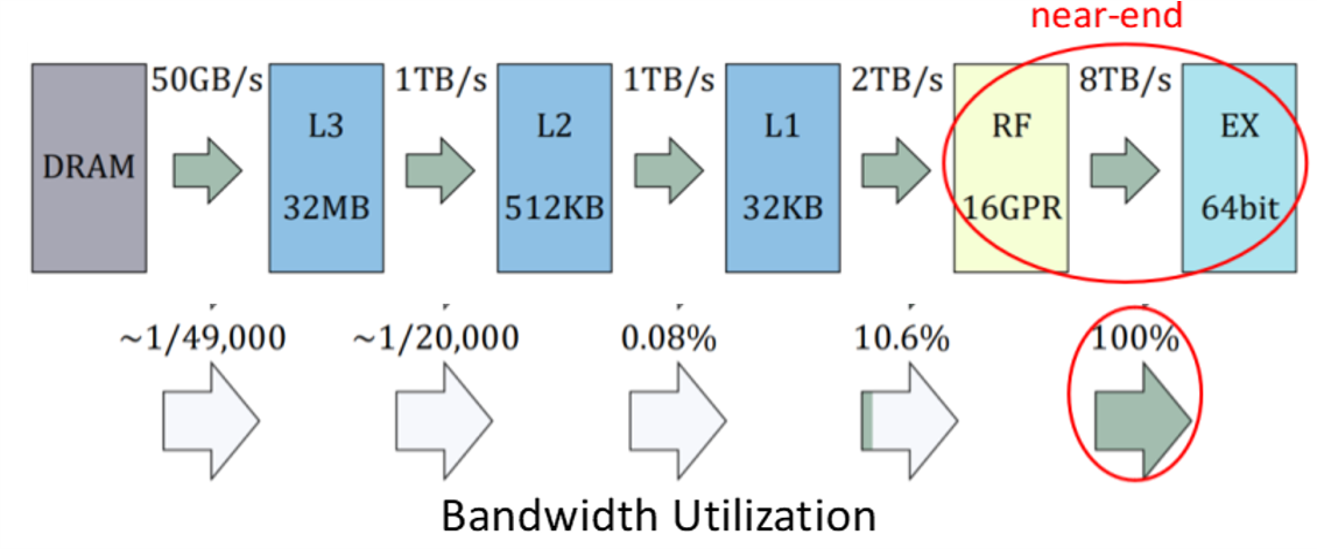
We analyzed the application characteristics of high-precision numerical computing and found that there is an “anti-memory wall” phenomenon: data transmission bottlenecks always appear at the near-computing storage hierarchy. This is because the data locality of numerical multiplication is so strong. If the word length natively supported by the computing device is not long enough, the operation needs to be decomposed into limbs, resulting in a huge amount of intermediate result memory access requests. Therefore, the new architecture must have: 1. The ability to process numerical multiplication; 2. The ability to process larger limbs at one time; 3. The ability to efficiently process large amounts of low-precision data.

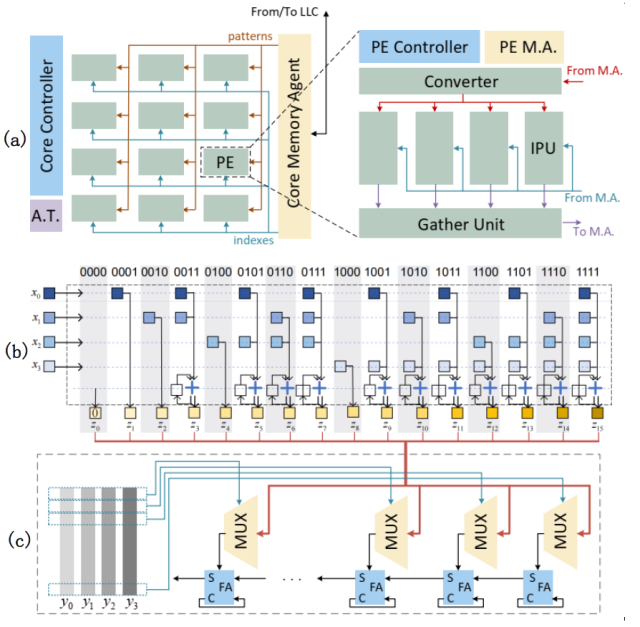
Addressing these requirements, we designed the Cambricon-P architecture.

The Cambricon-P architecture has the following features:

• Use bitflow to support high-precision numerical multiplication and low-precision linear algebra operations at the same time;
• The carry-select mechanism alleviates the strong data dependence in the multiplication algorithm to a certain extent, and achieves sufficient hardware parallelism;
• Bit-indexed inner product algorithm decomposes the calculation process into single-bit vectors, exploits the redundant computing hidden in finite field linear algebra, and reduces the computing logic required to 36.7% of the trivial method.

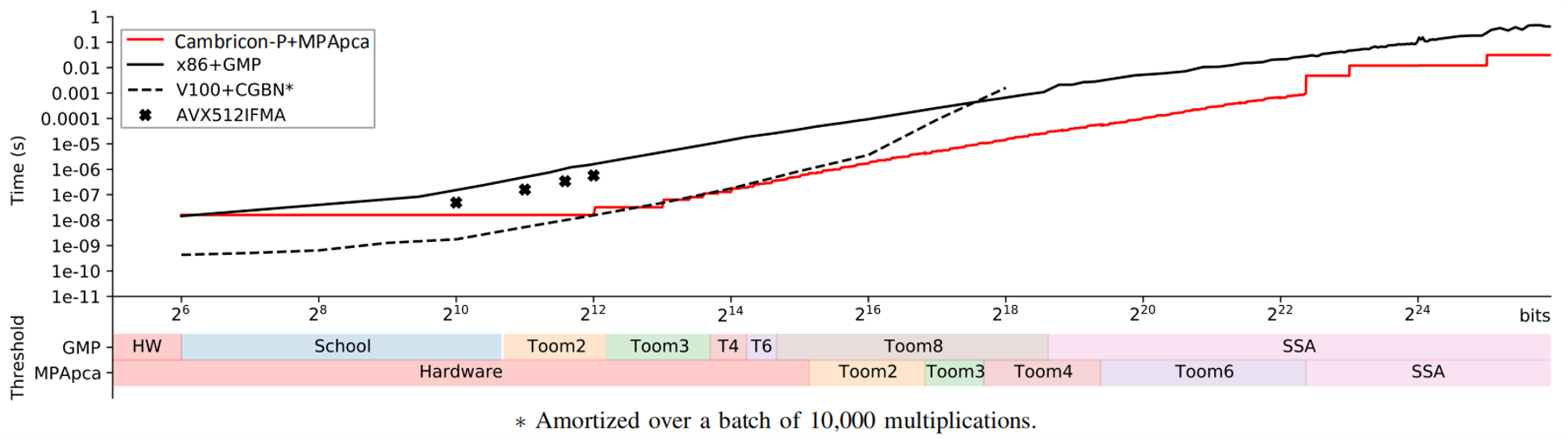
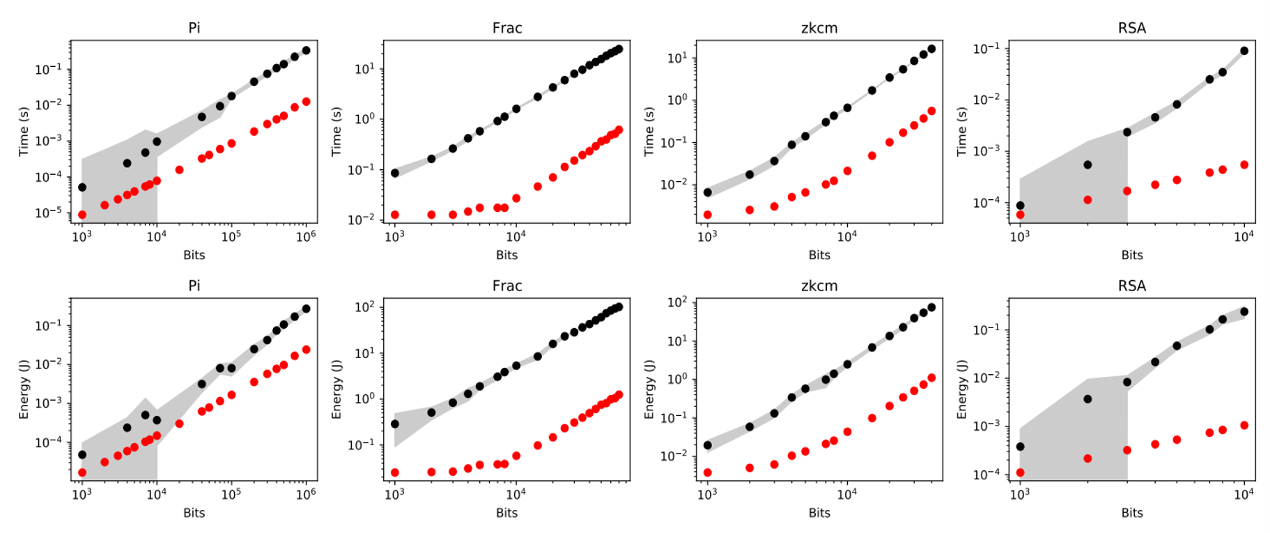
In order to achieve a larger-scale architecture and support larger limbs, the overall architecture of Cambricon-P is designed in a fractal manner, reusing the same control structure and similar data flows at the Core level, the Processing Element (PE) level, and the Inner Product Unit (IPU) level. We draftly developed the computing library MPApca for the Cambricon-P prototype, which implemented the Toom-Cook 2/3/4/6 fast multiplication algorithm and the Schönhage–Strassen fast multiplication algorithm (SSA) to evaluate against existing HPC systems such as CPU+GMP, GPU+CGBN.

Experimental results show that MPApca achieves up to 100.98x speedup compared to GMP in a monolithic multiplication, and achieves on average 23.41x speedup, 30.16x energy efficiency improvement in four typical applications.

Published on MICRO 2022. [DOI] [PDF]

Since starting from 1968, there are 1,900+ papers accepted on MICRO. Cambricon-P is awarded as Best Paper Runner-up, resulting in as the 4th nominee from China mainland institutes.

Invited by Prof. LI, Chao of SJTU, I attended the 1st CCF Chips conference, and gave an online talk to the session of Outstanding Young Scholars in Computer Architecture. In the talk I shared the results and extra thoughts from a paper under (single-blind) review, Rescue to the Curse of Universality. Since the results are still undergoing peer review, the points are for reference only.

UPD: Paper published on SCIENCE CHINA: Informational Sciences. [DOI] [PDF]

Take home messages:

• The Curse: It is impossible to build a computer that is both universal and efficient in logic circuits.
• REnc Architecture: It is sufficient to be an efficient architecture that taking the locality as a scale-invariant constraint.
• The results suggest that today’s DSAs may be over-specialized. There are theoretical rooms of universality while keeping the efficiency optimal.

With the laws from the semiconductor industry, we predict that DLPs are going to be more universal, more applicable, more standarized, and more systematic.

(The talk is only given in Mandarin currently.)

I have met JI, Yu, another CCF distinguished doctoral thesis award recipient, in Xining. He is very confused about my doctoral thesis: How could you make such a complex system into fractals? You really did that at Cambricon? I explained to him that fractalness is very primitive, rather than being made by me for thesis writing. In the talkshow of the day, I redefined the concept of Fractal Parallel Computing: Fractalness (parallel computing) is the primitive property of parallel computed problems, that there exists a finite program to control the arbitrarily scaled parallel machines, and to solve the problem of any size in finite time.

It is not only Doctor JI. Many peers have raised similar concerns. Indeed, it is showing that my works are still very preliminary. I must admit that fractal machines are yet hardly useful in practice to any other developers. But take an advice from me surely: if your system is not fractal, you should be really very cautious!

Allowing separate programming over a parallel machine can make the situation awkward: The excessive programs serve as advice strings to the computation.

Take an MPMD model for example. Since I have nodes to program and work in parallel, I can hardcode one bit of information into each node. At the very begining of the computation, I can gather the bits, forming an -bit natural number and distribute it to all nodes. Let us denote that number as . Trivially, can represent values up to .

Why would that matters? is smuggled into the programs, which depends on the scale of the parallel machine, which is further scalable with the problem size , thus introduced non-uniformity. Say, we let indicate the number of Turing Machines of descriptive size that halt on empty tapes. Then we get the following algorithm immediately:

0. Input as the description of a TM ( bit).
1. Gather and distribute the value of .
2. .
3. Parallel-for each :
   1. Simulate on an empty tape until halting.
   2. Increase atomically.
   3. If , abort the parallel for.
4. Return whether the -th simulation is finished or aborted.

It decides the Halting problem in finite time.

If your system does not allow that (deciding non-recursive problems), it is already fractal, although not necessarily in the identical form as in my thesis. The fundamental problem is that, the excessive programs are harmful. Theoretically they cause the non-computable problems being computable on your system; Practically they raise various problems, including the rewriting every year problem we encountered in Cambricon (Cambricon-F: Machine Learning Computers with Fractal von Neumann Architecture). Fractal computing systems are against these bad practices.

I hope the above argument makes the point clear.

Reference

• Pekka Orponen, Ker-i Ko, Uwe Schöning, and Osamu Watanabe. 1994. Instance complexity. J. ACM 41, 1 (Jan. 1994), 96–121.

When I was working on Cambricon-Q: A Hybrid Architecture for Efficient Training last year, I found that many graduate students do not know how to estimate errors, nor did they realize that error estimation is needed in randomized experiments. The computer architecture community does not pay enough attention to this. When performing experiments, our colleagues often run and measure a program of around ten milliseconds on the real system with the linux time command, and then report the speedup ratio compared with the simulation results. Such measurements are erroneous, and the results often fluctuate within a range; when the speedup is up to hundreds, a small measuring error may result in a completely different value in the final report. In elementary education, the experimental courses will teach us to “take the average of multiple measurements”, but how many times should “multiple times” be? Is 5 times enough? 10 times? 100 times? Or do you keep repeating it until the work is due? We need to understand the scientific method of experimentation: error estimation in repeated random experiments. I’ve found that not all undergraduate probability theory courses teach this, but it’s a must-have skill for a career in scientific research.

I am not a statistician, and I was also awful at courses when I was an undergraduate, so I am definitely not an expert in probability theory. But I used to delve into Monte Carlo simulation as a hobby, and I’m here to show how I did it myself. Statisticians, if there is a mistake, please correct me.

Gaussian Estimation

We have a set of samples , now assume that they are independent and identically distributed (i.i.d.), subject to a Gaussian distribution .

Although there is in the Gaussian distribution parameters, which is what we want, is not directly reflected in the measured samples. To approximate , we can take the arithmetic mean of the measured sample values. We first sum to get , then divide by . We get the arithmetic mean . Note that when a Gaussian random variable is divided by , the variance will be reduced by a factor of accordingly.

Although the above argument first assumes a Gaussian distribution, according to Levy-Lindeberg Central Limit Theorem (CLT), the infinite sum of any random variable tends to follow a Gaussian distribution, as long as those random variables satisfy the following two conditions:

• Finite variances;
• Independence.

So we can derive the distribution of directly from the CLT, no matter what distribution the samples actually follow, and the distribution is the same Gaussian. As long as there are enough samples, will converges to .

The Gaussian distribution tells us that we are 99.7% confident that the difference between and the true value we want is no more than three times the standard deviation, i.e., . We say that the confidence interval for the 99.7% confidence level of estimated is . As the number of experiments increases, the standard deviation of will continue to reduce. Originally we only knew that averaging over multiple measurements would work, and now we also know the rate of convergence: for every 4x more samples, the error will shrink by a factor of 2.

The constants 3 and 99.7% we use are a well known point on the Cumulative Distribution Function (CDF) of the Gaussian distribution, obtained by table look-up. Similar common values are 1.96 and 95%. To calculate the confidence level from the predetermined confidence interval, we use the CDF: , where the CDF only excludes the right-side tail, while the interval we estimate is two-sided, so the confidence level should subtract the left-side tail, i.e., . If you want to calculate the confidence interval from the target confidence level, you need to use the inverse function of CDF (ICDF), also known as PPF.

When programming, the CDF of the Gaussian distribution can be implemented relatively straightforward with the math library function erf. Its inverse function erfinv is not common, as it does not exist in the standard library of C or C++. However, CDF is continuous, monotonic, and derivable. Its derivative function is the Probability Density Function (PDF), so use numerical methods such as Newton’s method, secant, and bisection can all be applied for inversion efficiently.

However, the above estimation is entirely dependent on the CLT, which after all only describes a case in limits. In the actual experiment, we took 5 and 10 experimental results, which is far from the infinite number of experiments assumed. Do we still apply CLT though? This is obviously not scientific.

Student t-distribution

There is a more specialized probability distribution, the Student t-distribution, to define the sum of finitely many samples from random experiments. In addition to the above Gaussian estimation process, the t-distribution also considers the difference between the observed variance and the true variance .

The t-distribution is directly related to the degrees of freedom, which can be understood as in repeated random experiments. When the degrees of freedom are low, the tails of the t-distribution are longer, leading to a more conservative error estimate; as the degrees of freedom approach infinity, the t-distribution converges to a Gaussian distribution. For example, 5 samples, 4 degrees of freedom, and 99.7% confidence level, Gaussian estimated 3 times the standard deviation, while the t-distribution estimated 6.43 times, which is significantly enlarged.

When the number of trials is small, we use t-distribution instead of Gaussian distribution to describe . Especially when relying on error estimates to determine the early termination of repeated experiments, the use of Gaussian estimates is more prone to premature termination (especially when the first two or three samples happen to be similar).

Implementation

In Python, use packages: for Gaussian estimators use scipy.stats.norm.cdf and scipy.stats.norm.ppf, and for Student t-distribution estimators use scipy.stats.t.cdf and scipy.stats.t.ppf.

It is more difficult to implement in C++, the STL library is not fully functional for statistics, and it is inconvenient to introduce external libraries. The code below gives a C++ implementation of the two error estimators. The content between the two comment bars can be extracted as a header file for use, and the following part shows a sample program: Repeat experiments on until there is a 95% confidence that the true value will be included within plus or minus 10% of the estimated value.

Due to the emerging deep learning technology, deep learning tasks evolve toward complex control logic and frequent host-device interaction. However, the conventional CPU-centric heterogenous system has high host-device interaction overhead and slow improvement in interaction speed. Eventually, this leads to the problem of “interaction wall”, a gap between the improvement of interaction speed and the improvement of device computing speed. According to Amdahl’s law, this would severely limit the application of accelerators.

Addressing this problem, the CPULESS accelerator proposes a fused pipeline structure, which makes deep learning processor the center of the system, eliminating the need for an discrete host CPU chip. With the exception-oriented programming, the DLPU-centric system can combine the scalar control unit and the vector operation unit, and interaction overhead in between is minimized.

Experiments show that on a variety of emerging deep learning tasks with complex control logic, the CPULESS system can achieve 10.30x speedup and save 92.99% of the energy consumption compared to the conventional CPU-centric discrete GPU system.

Published in “IEEE Transactions on Computers”. [DOI] [PDF] [Artifact]

The pageview counter designed for this site, i.e., the one at the footer. I estimate that 99% of people nowadays use Python when dealing with MNIST. But this site promises not to use Python, thus chooses C++ for this gadget. The overall experience is not much complicated than Python, while it is expected to save a lot of carbons😁.

Implementation

Download MNIST testset and uncompress by gzip. LeCun said that the first 5k images are easier, so the program only use the first 5k images. Counter is saved into a file fcounter.db. Digits are randomly chosen from test images, assembled into one PNG image, (with Magick++ which is easier), then returned to the webserver via FastCGI.

The code is put in public domain now.

Compilation

• Install APT packages libmagick++-dev libfcgi-dev.
• For FastCGI++, compiler flags -lfcgi++ -lfcgi are required.
• CMake can found Magick++ automatically. Otherwise, append compiler flags from magick++-config.

Deployment

I use spawn-fcgi to spawn the compiled binary (set as a service in systemd). Most webservers support FastCGI, a reverse proxy to the port set by spawn-fcgi completes the deployment. I use Caddy:

1
2
3

reverse_proxy /counter.png localhost:21930 {
  transport fastcgi
}

Add /counter.png to the footer HTML, then you see digits bump on refresh. Go through internal links will not bump if the explorer cached the image.

In order to pursue energy efficiency, most deep learning accelerators use 8-bit or even lower bit-width computing units, especially on mobile platforms. Such low-bit-width accelerators can meet the accuracy requirements of inference tasks with special technical means, but they cannot be used during training, because the numerical sensitivity of the training process is much higher. How to extend the architecture to enable efficient mobile training?

In response to this problem, we proposed Cambricon-Q.

Cambricon-Q has introduced three new modules:

• SQU supports on-the-fly statistics and quantization;
• QBC manages the mixed precision and data format for the on-chip buffers;
• NDPO performs the weight update process at the near memory end.

The proposed architecture can support a variety of quantization-aware training algorithms. Experiments show that Cambricon-Q achieves efficient training with negligible accuracy loss.

Published on ISCA 2021. [DOI] [PDF]

This work follows Cambricon-F: Machine Learning Computers with Fractal von Neumann Architecture.

Cambricon-F obtains the programming scale-invariant property via fractal execution, alleviating the programming productivity issue of machine learning computers. However, the fractal execution on this computer is by the hardware controller and only supports a few common basic operators (convolution, pooling, etc.). Other functions need to be built on the sequence of these operators. We have found that when a limited and fixed instruction set is used to support complex and variable application payloads, inefficiency will occur.

When supporting regular algorithms such as conventional CNNs, the machine can achieve optimal efficiency. However, in complex and variable application scenarios, even if the application itself conforms to the definition of fractal operation, it will cause inefficiency phenomenon. The inefficiency phenomenon is defined as a suboptimal computational or communication complexity when certain applications are executed on a fractal computer. This paper uses TopK and 3DConv to illustrate the inefficiency phenomenon.

An intuitive example: The user wants to execute the application Bayesian Network, which conforms to the definition of fractal operation and can be executed efficiently in a fractal manner; But because there is no such “Bayesian” instruction in Cambricon-F, the application can only be decomposed into a series of basic operations and then executed serially. If the instruction set can be expanded, and a BAYES fractal instruction is added, the fractal execution can be maintained until the leaf node is reached, which significantly improves the computational efficiency.

Based on this, we improved the architecture of Cambricon-F and proposed Cambricon-FR with a fractal reconfigurable instruction set structure. Analytically, Cambricon-F is a Fractal Machine, while Cambricon-FR can be seen as a Universal Fractal Machine; Cambricon-F can achieve optimal efficiency on a specific application payload, while Cambricon-FR can achieve optimal efficiency on complex and variable application payloads.

Published in “IEEE Transactions on Computers”. [DOI] [PDF]

During the work as a software architect in the Cambricon Tech, I deeply realized the pain points of software engineering. When I first took over in 2016, the core software was developed by me and WANG Yuqing, with 15,000 lines of code; when I left in 2018, the development team increased to more than 60 people, with 720,000 lines of code. From the perspective of lines, the complexity of software doubles every 5 months. No matter how much manpower is added, the team is still under tremendous development pressure: customer needs are urgent and need to be dealt with immediately; New features need to be developed, the accumulated old code needs to be refactored; the documentation has not yet been established; the tests have not yet been established…

I may not be a professional software architect, but who can guarantee that the future changes are foreseen from the very beginning? Just imagine: the underlying hardware was single-core; it became multi-core a year later; then it became NUMA another year later. With such a rapid evolution, how can the same software be able to keep up without undergoing thorough refactoring? The key to the problem is that, the scale of the hardware has increased, so the level of abstraction that needs to be programmed and controlled is also increasing, making programming more complicated. We define the problem as the programming scale-variance.

In order to solve this problem from engineering practices, we started the research, namely Cambricon-F.

Addressing the scale-variance of programming, it is necessary to introduce some kinds of scale invariants. The invariant we found is fractal: the geometric fractals are self-similar on different scales. We define the workload in a fractal manner, so does the hardware architecture. Both scale invariants can be zoomed freely until a scale that is compatible with each other is found.

Cambricon-F first proposed the Fractal von Neumann Architecture. The key features of this architecture are:

• Sequential code, parallel execution adapted to the hardware scale automatically;
• Programming Scale-invariance: hardware scale is not coded, therefore code transfers freely between different Cambricon-F instances;
• High efficiency retained by fractal pipelining.

Published on ISCA 2019. [DOI] [PDF]